Quantum Variational Formula Explained with Examples

What Is the Quantum Variational Formula?

In essence, the quantum variational formula is a principle of approximation: it states that the lowest eigenvalue of a Hermitian operator (typically a Hamiltonian) is less than or equal to the expectation value of that operator to any quantum state.

Formally:

 

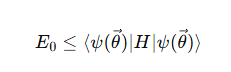
Where:

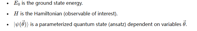
This forms the basis of the Variational Principle in quantum mechanics and is used to approximate ground states by minimizing the expectation value to θ

 

 

Why Quantum Variational Formula Matters in Quantum Computing

The quantum variational formula is the core theoretical engine behind Variational Quantum Algorithms (VQAs), such as:

• Variational Quantum Eigensolver (VQE)
• Quantum Approximate Optimization Algorithm (QAOA)
• Variational Quantum Classifier (VQC)

These algorithms:

• Are suitable for Noisy Intermediate-Scale Quantum (NISQ) devices.
• Use classical optimizers to iteratively tune a parameterized quantum circuit.
• Are flexible enough to target a wide range of quantum problems, including molecular simulations, optimization, and machine learning tasks.

How Quantum Variational Formula Works: Step-by-Step

1. Choose a Hamiltonian H

Usually derived from a problem (e.g., electronic structure of a molecule in chemistry).

2. Select an Ansatz ∣ψ(θ)⟩

This is a parameterized quantum circuit (e.g., UCCSD, hardware-efficient, or problem-inspired).

3. Evaluate the Expectation Value

Run the quantum circuit to compute ⟨ψ(θ)∣H∣ψ(θ)⟩ via repeated measurements.

4. Minimize Classically

Use classical optimization (e.g., COBYLA, SPSA, Adam) to adjust θ and minimize the expectation.

Applications of the Quantum Variational Formula

Quantum Chemistry

• Find ground-state energies of molecules.
• Predict chemical reactions and molecular bonding.
• Simulate strongly correlated systems beyond classical reach.

Materials Science

• Understand phase transitions in quantum systems.
• Model low-energy spectra of solids.

Machine Learning

• Optimize quantum classifiers with variational circuits.
• Implement quantum neural networks and feature maps.

Optimization

• Solve combinatorial problems like Max-Cut, TSP, portfolio optimization using QAOA variants.

Current Challenges of the Quantum Variational Formula

• Ansatz design: Choosing circuits expressive enough yet hardware-efficient.
• Barren plateaus: Gradients vanish in high-dimensional landscapes, slowing learning.
• Hardware noise: Quantum decoherence can affect the fidelity of expectation values.
• Scalability: Classical optimization becomes expensive as qubit count increases.

Future Directions of the Quantum Variational Formula

• Adaptive ansätze like ADAPT-VQE to reduce circuit depth dynamically.
• Noise-aware optimization techniques tailored for real devices.
• Hardware-algorithm co-design: Tightly integrating variational methods with specific quantum architectures.
• Quantum-aware machine learning: Embedding variational models into deep quantum pipelines.

Conclusion

The quantum variational formula isn't just a theoretical principle—it's a practical foundation powering some of the most promising quantum algorithms today. By enabling the collaboration between quantum and classical computing, it bridges the gap between NISQ devices and real-world applications.

As quantum hardware matures, the variational framework will evolve from approximation to precision science, shaping the future of computation, chemistry, and artificial intelligence.